Building Online Interactive Simulators for Predictive Models in R
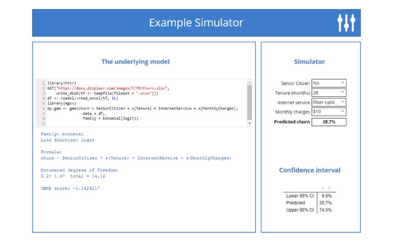
Correctly interpreting predictive models can be tricky. One solution to this problem is to create interactive simulators, where users can manipulate the predictor variables and see how the predictions change. This post describes a simple approach for creating online interactive simulators. It works for any model where there is a predict method. Better yet, if the model's not top secret, you can build and share the model for no cost, using the free version of Displayr!
In this post I show how to describe the very simple simulator shown below. Click the image to interact with it, or click the button below to explore and edit the code.
Explore and edit this simulator
Step 1: Create the model
The first step is to create a model. There are lots of ways to do this, including:
- Creating the model using R code from within Displayr. I illustrate this below.
- Pasting in estimates that you have already computed (Insert > Paste Table).
- Using Displayr's graphical user interface.
- Creating an R model somewhere else, saving it somewhere on the web (e.g., Dropbox), and then reading it into Displayr using readRDS. (See How to Link Documents in Displayr for a discussion of some utilities we have created for reading from Dropbox.)
In this post I will illustrate by using one of my all-time favorite models - a generalized additive model - via the gam function in the mgcv package. The process for creating this in Displayr is:
- Log in to Displayr (if you don't already have an account, click the GET DISPLAYR FREE button at the top-right of the screen).
- Press Insert > R Output (Analysis).
- Enter your code into the R Output and press the CALCULATE button at the top of the Object Inspector. In the example below I have fitted a GAM using some of IBM's telco churn example data.
Step 2: Add controls for each of the predictors
- Press Insert > Control (More) (this option is on the far right of the ribbon).
- In the Object Inspector > Properties > GENERAL, set the Name to cSeniorCitizen. You can give it any name you wish, but it is usually helpful to have a clear naming standard. In this example, I am using c so that whenever I refer to the control in code it is obvious to me that it is a control.
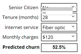
- Click on the Control tab of the Object Inspector and set the Item list to No; Yes, which means that the user will have a choice between No and Yes when using the control.
- Press Insert > Text box and click and drag to draw a text box to the left of the control. Type Senior Citizen into the text box, set it to be right-aligned (in the Appearance tab of the ribbon), with a font size of 10. You can micro-control layout by selecting the textbox, holding down your control key, and clicking the arrow keys on your keyboard.
- Click on the control and select No. It should look as shown below.
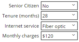
- Now, using shift and your mouse, select the text box and the control and press Home > Duplicate, and drag the copies to be neatly arranged underneath. Repeat this until you have four sets of labels and controls, one under each other.
- Update the textboxes, and each control's Name, and Item list, as follows:
- Tenure (months), cTenure: 0; 1; 2; 3; 4; 5; 6; 7; 8; 9; 10; 11; 12; 13; 14; 15; 16; 17; 18; 19; 20; 21; 22; 23; 24; 25; 26; 27; 28; 29; 30; 31; 32; 33; 34; 35; 36; 37; 38; 39; 40; 41; 42; 43; 44; 45; 46; 47; 48; 49; 50; 51; 52; 53; 54; 55; 56; 57; 58; 59; 60; 61; 62; 63; 64; 65; 66; 67; 68; 69; 70; 71; 72
- Internet service, cInternetService: No; DSL; Fiber optic
- Monthly charges, cMonthlyCharges: $0; $10; $20; $30; $40; $50; $60; $70; $80; $90; $100; $110; $120
- Select any option from each of the controls (it does not matter which you choose).
Step 3: Computing the prediction
Press Insert > R Output (Analysis) and then enter the code below, modifying it as per your needs. For example, with the code SeniorCitizen = cSeniorCitizen, the variable name used in the model is SeniorCitizen and cSeniorCitizen is the name of the control.
The item names in the control must exactly match the values of the variables in the data set. It is for this reason that the MonthlyCharges code is a bit more complicated, as it needs to strip out the $ from the control and convert it into a number (as the variable in the data set just contains numbers).
predict(my.gam,
        type = "response",
        newdata = data.frame(SeniorCitizen = cSeniorCitizen,
                    Tenure = as.numeric(cTenure),
                    InternetService = cInternetService,
                    MonthlyCharges = as.numeric(gsub("\\$", "", cMonthlyCharges))))[1] * 100
Confidence bands
Provided that the predict method supports them, the same approach easily extends to computing confidence intervals and other quantities from models. This code snippet computes the confidence intervals for the GAM used above.
pred <- predict(my.gam,
        se.fit = TRUE,
        newdata = data.frame(SeniorCitizen = cSeniorCitizen,
                    Tenure = as.numeric(cTenure),
                    InternetService = cInternetService,
                    MonthlyCharges = as.numeric(gsub("\\$", "", cMonthlyCharges))))
bounds = plogis(pred$fit + c(-1.96, 0, 1.96) * pred$se.fit) * 100
names(bounds) = c("Lower 95% CI", "Predicted", "Upper 95% CI")
bounds
Computing predictions from coefficients
And, of course, you can also make predictions directly from coefficients, rather than from model objects. For example, the following code makes a prediction for a logistic regression:
coefs = my.logistic.regression$coef
XB = coefs["(Intercept)"] +
        switch(cSeniorCitizen,
               No = 0,
               Yes = coefs["SeniorCitizenYes"]) +
        as.numeric(cTenure) * coefs["Tenure"] +
        switch(cInternetService,
               No =  coefs["InternetServiceNo"],
               "Fiber optic" = coefs["InternetServiceFiber optic"],
               DSL = 0) +
        as.numeric(gsub("\\$", "", cMonthlyCharges)) * coefs["MonthlyCharges"]
100 / (1 + exp(-XB))
Making safe predictions
Sometimes models perform "unsafe" transformations of the data in their internals. For example, some machine learning models standardize inputs (subtract the mean and divide by standard deviation). This can create a problem at prediction time, as the predict method may, in the background, attempt to repeat the standardization using the data for the prediction. This will cause an error (as the standard deviation of a single input observation is 0). Similarly, it is possible to create unsafe predictions from even the most well-written model (e.g., if using poly or scale in your model formula). There are a variety of ways of dealing with unsafe predictions, but a safe course of action is to perform any transformations outside of the model (i.e., not in the model formula).
Step 4: Export the simulator
If everything has gone to plan you can now use the simulator. To export it so that others can use it, click Export > Web Page, and you can then share the link with whoever you wish. The version that I have created here is very simple, but you can do a lot more if you want to make something pretty or more detailed (see the Displayr Dashboard Showcase for more examples).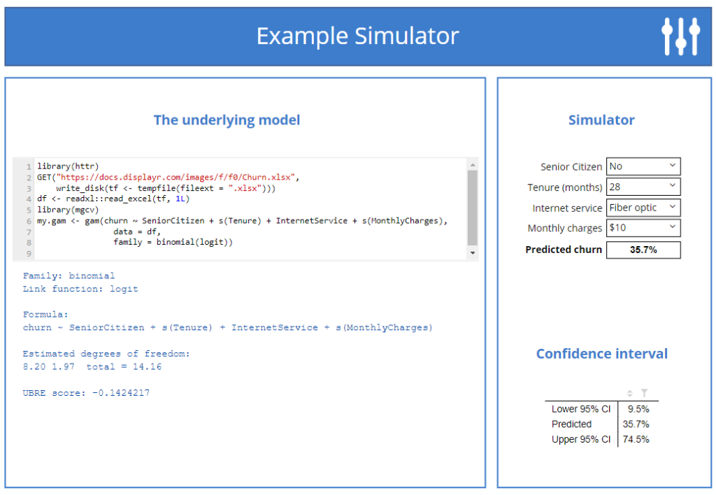
Explore and edit this simulator
Click here to interact with the published dashboard, or click here to open a copy of the Displayr document that I created when writing this post. It is completely live, so you can interact with it. Click on any of the objects on the page to view the underlying R code, which will appear in the Object Inspector > Properties > R CODE.
Ready to get started? Create your own simulator for free in Displayr!

